Linear Programming
Linear
programming (LP) is a specific type of optimization that help users determine
the optimal allocation of scarce resources in order to maximize profits,
minimize costs, obtain the best possible quality etc. It is applicable in a wide
variety of business areas for solving allocation problems. Some of the most
typical ones are production planning, workforce scheduling, financial portfolio
optimization and capital budgeting.
A linear programming problem contains
an objective function and a set of constraints, all of which are linear. The
problem is finding the best combination of activity levels, without using more
resources than are actually available.
Among many software packages that are
dedicated to solving linear programs, Microsoft Excel spreadsheet with its
Solver add-in is the one that we are focusing on. For illustrating formulation
of problems as LP models, solving them and interpreting the results, a product
mix problem (Example 3.1) would be pretty helpful.
Product-Mix Problem
The Monet Company produces four types of picture frames. Each type requires different amounts of skilled labor, metal and glass; and is sold for a different price. Given the limited amounts of these inputs, Monet wants to create a production plan that will maximize weekly profits, while only producing enough number of frames that can actually be sold. LP model will come up with the exact number of the four types of frames to be produced each week that will maximize weekly profits and that will meet the constraints at the same time.
Formulating
the Model:
A linear programming problem consists
of three parts, which are decision variables, the objective function and a set
of constraints.
-
Decision Variables
The first step of formulating a model is
identifying the decision variables. They are the controllable inputs of the
model describing the quantities that the decision makers want to find. Thus,
their values determine the solution of the model. In other words, they are the
unknowns of the model.
The decision variables are the number
of frames of type 1,2,3 and 4 to be produced, which are labeled x1,
x2, x3, and x4 respectively.
Decision Variables |
Label |
|
Number of type 1 frames to be produced |
X1 |
|
Number of type 2 frames to be produced |
X2 |
|
Number of type 3 frames to be produced |
X3 |
|
Number of type 4 frames to be produced |
X4 |
-
Objective Function
The next
step in formulating an LP model is defining the objective function, which must
be either maximization or minimization of a linear function. The objective
function depends on the decision variables and represents the goal of the
decision maker. For the Monet Company, the objective function is:
Maximizing 6 x1 + 2 x2 +
4 x3 + 3 x4
This means that Monet wants to find the number of
each type of frames to be produced, which gives the maximum value for weekly
profits. The coefficient of each decision variable in the objective function
represents the amount that each frame type contributes to profit, and it is
calculated as the unit selling price minus the cost of the inputs for a single
frame of each type. The total profit is obtained by adding up the profits from
the four products.
-Constraints
These are the real world limitations on
the decisions that come from the decision makers’ environment such as limited
resources, physical laws and contractual obligations. A constraint is an
equality or inequality that restricts the possible values a variable can take. Constraints
must be linear with the forms of ≤, ≥ or =. Strict inequalities
(< or >) are not permitted in an LP model.
The following inequalities restrict the
total number of labor hours that can be purchased to 4,000, the total ounces of
metal to 6,000 and the total ounces of glass to 10,000.
2 x1 + x2 +
3 x3 + 2 x4 ≤ 4,000 (labor constraint)
4 x1 + 2 x2 +
x3 + 2 x4 ≤ 6,000 (metal constraint)
6 x1 + 2 x2 + x3 +
2 x4 ≤ 10,000
(glass constraint)
The following market constraints
specify that it is impossible to sell more than 1,000 type 1 frames, 2,000 type
2 frames, 500 type 3 frames and 1,000 type 4 frames.
x1 ≤ 1,000 (frame 1 sales
constraint)
x2 ≤ 2,000 (frame 2 sales
constraint)
x3 ≤ 500 (frame 3 sales constraint)
x4 ≤ 1,000 (frame 4 sales
constraint)
Since producing a negative number of
products would make no sense, nonnegativity constraints should be added to the
LP model formula. The maximum sales constraints above and the nonnegativity
constraints below place upper and lower limits on the numbers of frames that
can be produced.
x1, x2,
x3, x4 ≥ 0
(nonnegativity constraints)
The resulting mathematical formulation of the linear
programming problem is:
maximize 6 x1 + 2
x2 + 4 x3 + 3 x4 subject to 2
x1 + x2
+ 3 x3
+ 2 x4 ≤ 4,000 4 x1 + 2 x2 + x3 + 2 x4 ≤ 6,000 6 x1 + 2 x2 + x3 + 2 x4 ≤ 10,000 x1 ≤ 1,000 x2 ≤ 2,000 x3 ≤ 500 x4 ≤ 1,000 x1, x2,
x3, x4 ≥
0
Developing the Spreadsheet Model:
Having formulated the problem, it is
time to enter them into Excel. The spreadsheet includes four sections that are
the inputs, production plan, constraints on inputs & revenue, and cost
summary.
- Input data
We start
with entering the input parameters into the cells, which are enclosed in a blue
border. These are the uncontrollable inputs of the model that are usually given
constant quantitative values. Therefore, only numbers, not formulas are entered
into input cells. In this problem, the uncontrollable inputs are the unit
costs, which are $8.00 per labor hour, $0.50 per ounce of metal and $0.75 per
ounce of glass. Other inputs are the certain amounts of skilled labor, metal
and glass required for each type of frames and their unit selling prices.
- Production plan
In this section, we enter any values
for each frame type. Although we can use any trial values, Solver will find the
optimal values that satisfy all constraints. These are the cells that include
the decision variables. The range is named “Produced”, and bordered by red.
In this section, we can also reflect
the sales constraints by entering the maximum units of frames that can be sold
and call this range “MaxSales”.
- Constraints on inputs
In this
section, we enter SUMPRODUCT function to calculate the units of labor, metal
and glass used by the current product mix, and name the range as “Used”. To the
right of the “Used” range, the maximum available limits of these resources are
entered and the region is labeled as “Available”.
- Revenue, cost summary
At the
bottom of the spreadsheet model, the revenues and costs associated with each
product is calculated to get the final outcome, total profit.
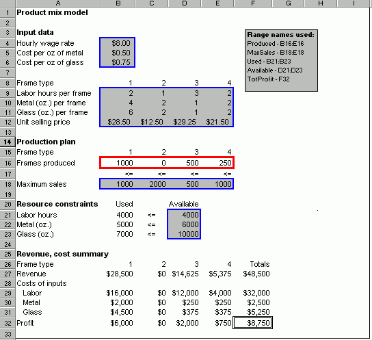
The following snapshot of the model
includes the results for trail production values of 1000 for frame 1, 0 for
frame 2, 500 for frame 3, and 250 for frame 4.
Obtaining Results using Solver:
Once the
model has been created, the next step is invoking Solver to specify the
changing cells for decision variables, the target cell and the constraints in
order to ask Solver to find the optimal quantity of each frame type to maximize
the weekly profit.
To let Solver know the cells on the
spreadsheet that represent the decision variables, objective function and
constraints, we open the Solver dialog box. The sections that must be filled in
are:
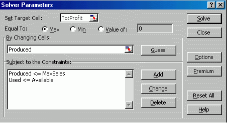
- Target cell: It contains the value of the
objective function that we want to maximize. Therefore, we enter the Total
Profit (TotProfit) cell as the target cell, and click on the “Maximize” button.
- Changing cells: These are the cells that contain the decision variables. Solver changes the values in these cells to optimize the objective
function. Therefore, we enter the “Produced” range, which includes the numbers
of frames to produce, as the changing cells.
- Constraints: To indicate that no more
of each resource can be used than is available, we add the constraint “Used
<= Available”. To specify that its maximum sales level is the upper limit on
the quantity of each frame type to be produced, we add the constraint “Produced <= MaxSales”.
When the parameters have been entered,
the Solver Parameters dialog box looks like:
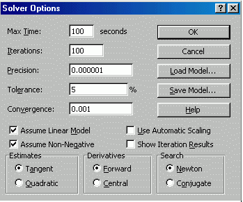
As the last step before clicking on
Solve button, we must specify that the changing cells must be kept nonnegative
by checking the “Assume Non-Negative” box in the Solver Options dialog box as
shown below. We also check the “Assume Linear Model” box to instruct Excel to
use the Simplex Method, which is the most efficient one for solving linear
models.
When we click on the “Solve” button in
the Solver Parameters dialog box, Solver finds the optimal solution by changing
the values for the decision variables, which are the number of each type of
frames to be produced. As shown in the following snapshot of the model, the
optimal production plan that maximizes weekly profit while satisfying the
constraints is to produce 1000 type 1 frames, 800 type 2 frames, 4000 type 3
frames and no type 4 frames.
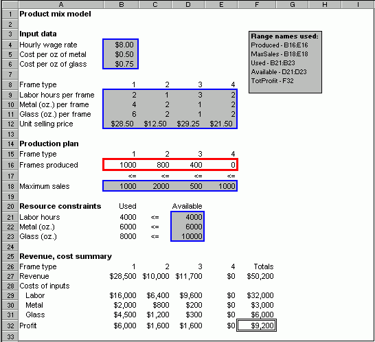
Monet utilizes all of the available
labor hours and metal but only 8,000 of the10,000 ounces of glass available and
earns $9,200 profit. Although it can still produce more type 2, 3 and 4 frames
to meet their maximum sales constraints, it does not have enough labor and
metal for production. Therefore, the labor hours and metal availability
constraint, since they are met exactly, are the bottlenecks for this situation and
are called binding constraints. This means if either the labor hours or metal
availability are increased, the profit would increase. The glass availability
constraint, since it has 2,000 units of slack, is the nonbinding constraint of
production.
The details of the optimum solution are
given in the Solver’s Answer Report below. The original trial values and the
final values of the objective function and the decision variables, as well as
the status of each constraint are provided.
|
|
|
|
|
|
|
|
|
|
|
|
|
|
Microsoft
Excel 9.0 Answer Report |
|
|
|
|
|||
|
|
|
|
|
|
|
|
|
|
|
|
|
|
Target
Cell (Max) |
|
|
|
|
|
||
|
|
|
|
Cell |
Name |
Original Value |
Final Value |
|
|
|
|
|
|
|
$F$32 |
TotProfit |
$8,750 |
$9,200 |
|
|
|
|
|
|
|
|
|
|
|
|
|
|
|
|
|
|
|
|
|
|
|
|
|
|
|
|
Adjustable
Cells |
|
|
|
|
|
||
|
|
|
|
Cell |
Name |
Original Value |
Final Value |
|
|
|
|
|
|
|
$B$16 |
Type 1 frames produced |
1000 |
1000 |
|
|
|
|
|
|
|
$C$16 |
Type 2 frames produced |
0 |
800 |
|
|
|
|
|
|
|
$D$16 |
Type 3 frames produced |
500 |
400 |
|
|
|
|
|
|
|
$E$16 |
Type 4 frames produced |
250 |
0 |
|
|
|
|
|
|
|
|
|
|
|
|
|
|
|
|
|
|
|
|
|
|
|
|
|
|
|
|
Constraints |
|
|
|
|
|
||
|
|
|
|
Cell |
Name |
Cell Value |
Formula |
Status |
Slack |
|
|
|
|
|
$B$21 |
Labor hours Used |
4000 |
$B$21<=$D$21 |
Binding |
0 |
|
|
|
|
|
$B$22 |
Metal (oz.) Used |
6000 |
$B$22<=$D$22 |
Binding |
0 |
|
|
|
|
|
$B$23 |
Glass (oz.) Used |
8000 |
$B$23<=$D$23 |
Not Binding |
2000 |
|
|
|
|
|
$B$16 |
Type 1 frames produced |
1000 |
$B$16<=$B$18 |
Binding |
0 |
|
|
|
|
|
$C$16 |
Type 2 frames produced |
800 |
$C$16<=$C$18 |
Not Binding |
1200 |
|
|
|
|
|
$D$16 |
Type 3 frames produced |
400 |
$D$16<=$D$18 |
Not Binding |
100 |
|
|
|
|
|
$E$16 |
Type 4 frames produced |
0 |
$E$16<=$E$18 |
Not Binding |
1000 |
|
|
|
|
|
|
|
|
|
|
|
|
Performing Sensitivity Analysis:
Sensitivity analysis can be performed
by clicking on “Sensitivity” in the dialog box that appears when Solver finds
the optimal solution to the problem:
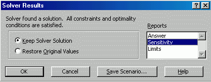
The resulting Sensitivity Report
provides information on reduced costs, shadow prices, the upper and lower
allowable limits for decision variables and constraints.
|
|
|
|
|
|
|
|
|
|
|
|
|
|
|
Microsoft
Excel 9.0 Sensitivity Report |
|
|
|
|
||||
|
|
|
|
|
|
|
|
|
|
|
|
|
|
|
Adjustable
Cells |
|
|
|
|
|
|
||
|
|
|
|
|
|
Final |
Reduced |
Objective |
Allowable |
Allowable |
|
|
|
|
|
Cell |
Name |
Value |
Cost |
Coefficient |
Increase |
Decrease |
|
|
|
|
|
$B$16 |
Type 1 frames produced |
1000 |
2 |
6 |
1E+30 |
2 |
|
|
|
|
|
$C$16 |
Type 2 frames produced |
800 |
0 |
2 |
1 |
0.25 |
|
|
|
|
|
$D$16 |
Type 3 frames produced |
400 |
0 |
4 |
2 |
0.5 |
|
|
|
|
|
$E$16 |
Type 4 frames produced |
0 |
0 |
3 |
0.2 |
1E+30 |
|
|
|
|
|
|
|
|
|
|
|
|
|
|
|
|
Constraints |
|
|
|
|
|
|
||
|
|
|
|
|
|
Final |
Shadow |
Constraint |
Allowable |
Allowable |
|
|
|
|
|
Cell |
Name |
Value |
Price |
R.H. Side |
Increase |
Decrease |
|
|
|
|
|
$B$21 |
Labor hours Used |
4000 |
1.20 |
4000 |
250 |
1000 |
|
|
|
|
|
$B$22 |
Metal (oz.) Used |
6000 |
0.40 |
6000 |
2000 |
500 |
|
|
|
|
|
$B$23 |
Glass (oz.) Used |
8000 |
0.00 |
10000 |
1E+30 |
2000 |
|
|
|
|
|
|
|
|
|
|
|
|
|
The first part of the report gives
information concerning the objective function. The allowable increase/decrease
represents the range in which the current solution remains optimal. We see that
the unit profit (the objective function coefficient) of type 1 frames would
have to decrease by $2.00 for the current product mix to change. The unit profit for type 2 frames can
range between $1.75 and $3.00, whereas that of type 3 can be between $3.50 and
$6.00 with the current product mix remaining optimal. But, the unit profit for
type 4 frames would have to increase by $0.20 before they can start to be
produced. It should also be noted that the ranges above are valid only if one
coefficient is altered at a time.
Reduced cost refers to the increase in profit by producing one more unit
of a product. Therefore, Monet’s profit can increase by $2 if it produces an
extra unit of Type 1 frames, whereas producing additional amounts of other
frame types would lead to no extra gains.
The second part of the sensitivity
report gives information about the constraints. The shadow price refers to the
marginal increase in profit by obtaining an extra unit of a resource. Therefore,
it is the maximum amount that the company is willing to pay for an extra unit.
We conclude that Monet is willing to pay $1.20 for each additional labor hour
between 3,000 and 4,250 hours, $0.4 for each extra ounce of metal between 5,500
and 8,000 ounces. Since glass is underutilized by 2,000 ounces, there is no
need for purchasing any additional units. Thus, its shadow price is $0.
To see the impact of changes in one or
more constraints on the optimal profit and the optimal product mix, we also
perform a sensitivity analysis by using the SolverTable add-in. To measure the
effect of a change in a single input on any number of outputs, a “one-way”
table is used. The impact of simultaneous changes in two inputs on one output
is determined by a “two-way” table.
To illustrate the use of SolverTable
for one-way sensitivity analysis, we can measure the sensitivity of outputs to
variations in the number of labor hours available. We start by selecting a
one-way table in the Data/SolverTable dialog box, and fill in the next dialog
box as shown below:
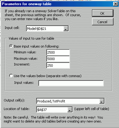
The cell including the number of labor hours available is
selected as the input cell. Then, the desired minimum and maximum values of
inputs are entered. At the bottom of the dialog box, we specify the number of
each type of frame to be produced and the total profit as the outputs.
SolverTable returns the following output table:
|
|
|
|
|
|
|
|
|
|
|
|
|
|
Sensitivity of optimal solution to number of labor hours |
|
|
|
||||
|
|
|
|
Frames produced
|
|
|
|
|||
|
|
|
Labor hours
|
1 |
2 |
3 |
4 |
Total profit |
|
|
|
|
|
|
$B$16 |
$C$16 |
$D$16 |
$E$16 |
$F$32 |
Increase |
|
|
|
|
2500 |
1000 |
500 |
0 |
0 |
$7,000 |
|
|
|
|
|
2750 |
1000 |
750 |
0 |
0 |
$7,500 |
$500 |
|
|
|
|
3000 |
1000 |
1000 |
0 |
0 |
$8,000 |
$500 |
|
|
|
|
3250 |
1000 |
950 |
100 |
0 |
$8,300 |
$300 |
|
|
|
|
3500 |
1000 |
900 |
200 |
0 |
$8,600 |
$300 |
|
|
|
|
3750 |
1000 |
850 |
300 |
0 |
$8,900 |
$300 |
|
|
|
|
4000 |
1000 |
800 |
400 |
0 |
$9,200 |
$300 |
|
|
|
|
4250 |
1000 |
750 |
500 |
0 |
$9,500 |
$300 |
|
|
|
|
4500 |
1000 |
500 |
500 |
250 |
$9,750 |
$250 |
|
|
|
|
4750 |
1000 |
250 |
500 |
500 |
$10,000 |
$250 |
|
|
|
|
5000 |
1000 |
0 |
500 |
750 |
$10,250 |
$250 |
|
|
|
|
|
|
|
|
|
|
|
|
We
can see that for any available labor hour values between 2,500 and 5,000, the quantity of type 1 frames to be
produced does not change. But, type 2
frames would be discontinued
if 5,000 labor hours were available. The production of type 3 frames would start at 3,250 labor hours and frames of type 4
would finally be produced when 4,500
labor hours are available.
In the last column of the table above, we can track how
labor hours increase the total profit. Although this is not automatically
produced by SolverTable add-in, we can easily compute it on the spreadsheet. It
is clear that having extra labor hours adds to profit. But the increase in
profit per extra hour, called the shadow price of labor hours, decreases as
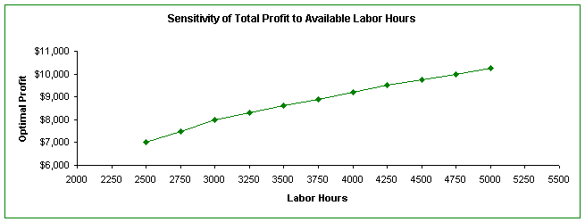
more hours are obtained. We can graph the optimal profit values versus the
available labor hours to display how shadow price, which is the slope of the
line, decreases as more labor hours are purchased.
